Introduction

In years 2018-2019, on behalf of the Italian Society of Human Genetics (SIGU) an itinerant Galaxy-based “hands-on-computer” training activity entitled “Data analysis and interpretation for clinical genomics” was held four times on invitation from different Italian institutions (Università Cattolica del Sacro Cuore in Rome, University of Genova, SIGU 2018 annual scientific meeting in Catania, University of Bari) and was offered to about 30 participants each time among clinical doctors, biologists, laboratory technicians and bioinformaticians. Topics covered by the course were NGS data quality check, detection of variants, copy number alterations and runs of homozygosity, annotation and filtering and clinical interpretation of sequencing results.

Realizing the constant need for training on NGS analysis and interpretation of sequencing data in the clinical setting, we designed an on-line Galaxy-based training resource articulated in presentations and practical assignments by which students will learn how to approach NGS data quality at the level of fastq, bam and VCF files and clinically-oriented examination of variants emerging from sequencing experiments.

This training course is not to be intended as a tutorial on NGS pipelines and variant calling. This on-line training activity is indeed focused on data analysis for clinical interpretation. If you are looking for training on variant calling, visit this Galaxy tutorial on Exome sequencing data analysis for diagnosing a genetic disease.

comment SIGU

The Italian Society of Human Genetics (SIGU) was established on November 14, 1997, when the pre-existing Italian Association of Medical Genetics and the Italian Association of Medical Cytogenetics joined. SIGU is one of the 27 member societies of FEGS (Federation of European Genetic Societies). Animated by a predominant scientific spirit, SIGU wants to be reference for all health-care issues involving human genetics in all its applications. Its specific missions are to develop quality criteria for medical genetic laboratories, to promote writing of guidelines in the field of human genetics and public awareness of the role and limitations of genetic diagnostic techniques. SIGU coordinates activities of several working groups: Clinical Genetics, Cytogenetics, Prenatal Diagnosis, Neurogenetics, Fingerprinting, Oncological Genetics, Immunogenetics, Genetic Counseling, Quality Control, Medical Genetics Services, Bioethics. More than 1000 medical geneticists and biologists are active members of the society.

Agenda

In this tutorial, we will cover:

1. Next Generation Sequencing
   1. NGS in the clinic
   2. Basics of NGS bioinformatic analysis
   3. Alignment
   4. Post-alignment BAM processing
   5. Variant calling
2. Requirements
3. Datasets
   1. Use cases
   2. Get data
4. Quality control
   1. Quality control of FASTQ files
   2. Quality control of BAM files
5. Variant annotation
   1. Gene model
   2. Sequence variant nomenclature
   3. Variant class
   4. Population sequencing db
   5. Variant-disease/gene-disease db
   6. Annotation Software and tools
   7. Annotation and filtering with SnpEFF
6. Variant prioritization
   1. Variant impact
   2. Variant frequency
   3. Variant effect prediction Tools
   4. ACMG/AMP 2015 guidelines
   5. Prioritization
   6. GEMINI for variant filtering
   7. Candidate variant detection
7. Solutions
8. Advanced analysis

Next Generation Sequencing

Next (or Second) Generation Sequencing (NGS/SGS) is an umbrella-term covering a number of approaches to DNA sequencing that have been developed after the first, widespread and for long time most commonly used Sanger sequencing.

NGS is also known as Massive Parallel Sequencing (MPS), a term that makes explicit the paradigm shared by all these technologies, that is to sequence in parallel a massive library of spatially separated and clonally amplified DNA templates.

For a comprehensive review of the different NGS technologies see Goodwin et al., 2016, which also includes an introduction to the third generation methods allowing sequencing of long single-molecule reads.

NGS in the clinic

In the span of less than a decade, NGS approaches have pervaded clinical laboratories revolutionizing genomic diagnostics and increasing yield and timeliness of genetic tests.

In the context of disorders with a recognized strong genetic contribution such as neurogenetic diseases, NGS has been firmly established as the strategy of choice to rapidly and efficiently diagnose diseases with a Mendelian basis. A general diagnostic workflow for these disorders currently embraces different NGS-based diagnostic options as illustrated in Figure 1.

---

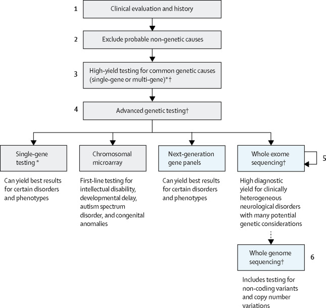
Figure 1. General workflow for genetic diagnosis of neurological diseases. (*If considering high-yield single-gene testing of more than 1–3 genes by another sequencing method, note that next-generation sequencing is often most cost-effective. †Genetic counselling is required before and after all genetic testing; other considerations include the potential for secondary findings in genomic testing, testing parents if inheritance is sporadic or recessive, and specialty referral.) From Rexach et al., 2019

---

Currently, most common NGS strategies in clinical laboratories are the so-called targeted sequencing methods that, as opposed to genome sequencing covering the whole genomic sequence, focus on a pre-defined set of regions of interest (the targets). The targets can be selected by hybrid capture or amplicon sequencing, and the target-enriched libraries is then sequenced. The most popular target designs are:

• gene panels where the coding exons of only a clinically-relevant group of genes are targeted
• exome sequencing where virtually all the protein-coding exons in a genome are simultaneously sequenced

Basics of NGS bioinformatic analysis

Apart from the different width of the target space in exome and gene panels, these two approaches usually share the same experimental procedure for NGS library preparation. After clonal amplification, the fragmented and adapter-ligated DNA templates are sequenced from both ends (paired-end sequencing) of the insert to produce short reads in opposite (forward and reverse) orientation.

Bioinformatic analysis of NGS data usually follows a general three-step workflow to variant detection. Each of these three steps is marked by its “milestone” file type containing sequence data in different formats and metadata describing sequence-related information collected during the analysis step that leads to generation of that file.

NGS workflow step	File content	File format	File Size (individual exome)
Sample to reads	Unaligned reads and qualities	fastQ	gigabytes
Reads to alignments	Aligned reads and metadata	BAM	gigabytes
Alignments to variants	Genotyped variants and metadata	VCF	megabytes

Here are the different formats explained:

• fastQ (sequence with quality): the de facto standard for storing the output of high-throughput sequencing machines
  • Usually not inspected during data analysis
• BAM (binary sequence alignment/map): the most widely used TAB-delimited file format to store alignments onto a reference sequence
  • Aligned reads
• VCF (variant call format): the standard TAB-delimited format for genotype information associated with each reported genomic position where a variant call has been recorded

Another useful file format is BED, to list genomic regions of interest such as the exome or panel targets.

The steps of the reads-to-variants workflow can be connected through a bioinformatic pipeline (Leipzig et al., 2017), consisting in read alignments, post-alignment BAM processing and variant calling.

Alignment

As generated by the sequencing machines, paired-end reads are written to two fastQ files in which forward and reverse reads are stored separately together with their qualities. FastQ files are taken as input files by tools (the aligners) that align the reads onto a reference genome. One of the most used aligners is BWA among the many that have been developed (Figure 2).

---

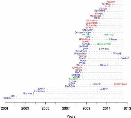
Figure 2. Aligners timeline 2001-2012 (from Fonseca et al., 2012)

---

During the bioinformatic process, paired-end reads from the two separate fastQ files are re-connected in the alignment, where it is expected that they will:

• map to their correct location in the genome
• be as distant as the insert size of the fragment they come from
• be in opposite orientations a combination which we refer to as proper pairing. All these data about paired-end reads mapping are stored in the BAM file and can be used to various purposes, from alignment quality assessment to structural variant detection.

In Figure 3, the Integrative Genomic Viewer (IGV) screenshot of an exome alignment data over two adjacent ASXL1 exons is shown. Pink and violet bars are forward and reverse reads, respectively. The thin grey link between them indicates that they are paired-end reads. The stack of reads is concentrated where exons are as expected in an exome, and the number of read bases covering a given genomic location e (depicted as a hill-shaped profile at the top of the figure) defines the depth of coverage (DoC) over that location:

DoC_e=number of read bases over e/genomic length of e

---

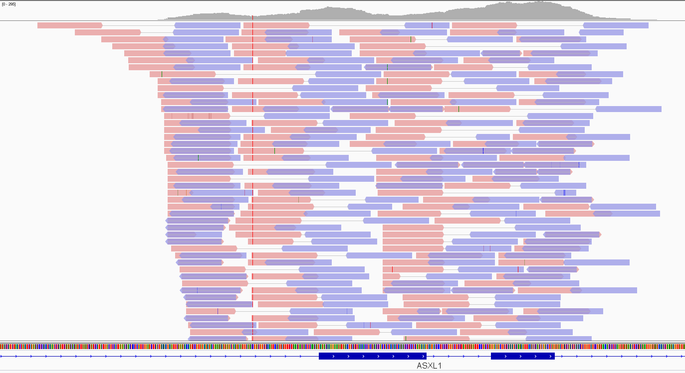Figure 3. Exome data visualization by IGV

---

Post-alignment BAM processing

Regarding post-alignment pipelines, the most famous for germline SNP and InDel calling is probably that developed as part of the GATK toolkit (Figure 4).

---

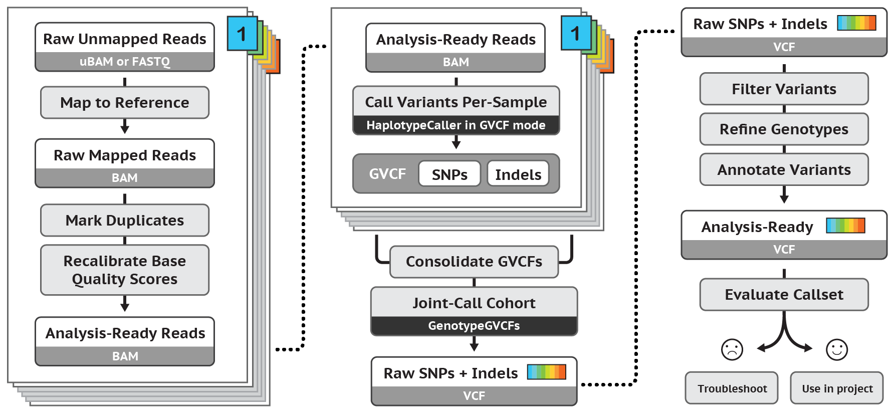
Figure 4. After-alignment pipeline for germline SNP and InDel variant calling according to GATK Best Practices

---

According to GATK best practices, in order to be ready for variant calling the BAM file should undergo the following processing:

• marking duplicate reads to flag (or discard) reads that are mere optical or PCR-mediated duplications of the actual reads
• recalibrating base quality scores to correct known biases of the native base-related qualities While GATK BAM processing is beyond doubt important to improve data quality, it has to be noticed that it is not needed to obtain variant calls and that non GATK-based pipelines may not use it or may use different quality reparametrization schemes. Duplicate flagging or removal is not recommended in amplicon sequencing experiments.

Variant calling

The process of variant detection and genotyping is performed by variant callers. These tools use probabilistic approaches to collect evidence that non-reference read bases accumulating over a given locus support the presence of a variant, usually differing in algorithms, filtering strategies, recommendations (Sandmann et al., 2017). To be confident that a variant is a true event, its supporting evidence should be significantly stronger than chance; e.g. the C>T on the left of the screenshot in Figure 5 is supported by all its position-overlapping reads, claiming for a variant. In contrast, the C>A change on the right of the screenshot is seen only once over many reads, challenging its interpretation as a real variant. In fact, DNA variants that occur in germ cells (i.e., germline/constitutional variants that can be passed on to offspring) are either diploid/biallelic, so expected alternative allele frequency is 50% for a heterozygous change. On the other hand, if only a smaller subset of aligned reads indicates variation, that could result from technology bias or be a mosaicism, i.e. an individual which harbour two or more populations of genetically distinct cells as a result of postzygotic mutation. Postzygotic de novo mutations may result in somatic mosaicism (potentially causing a less severe and/or variable phenotype compared with the equivalent constitutive mutation) and/or germline mosaicism (hence enabling transmission of a pathogenic variant from an unaffected parent to his affected offspring) (Biesecker et al., 2013). To identify mosaicism, a probabilistic approach should consider deviation of the proband variant allele fraction (VAF, defined as the number of alternative reads divided by the total read depth) from a binomial distribution centred around 0.5.

---

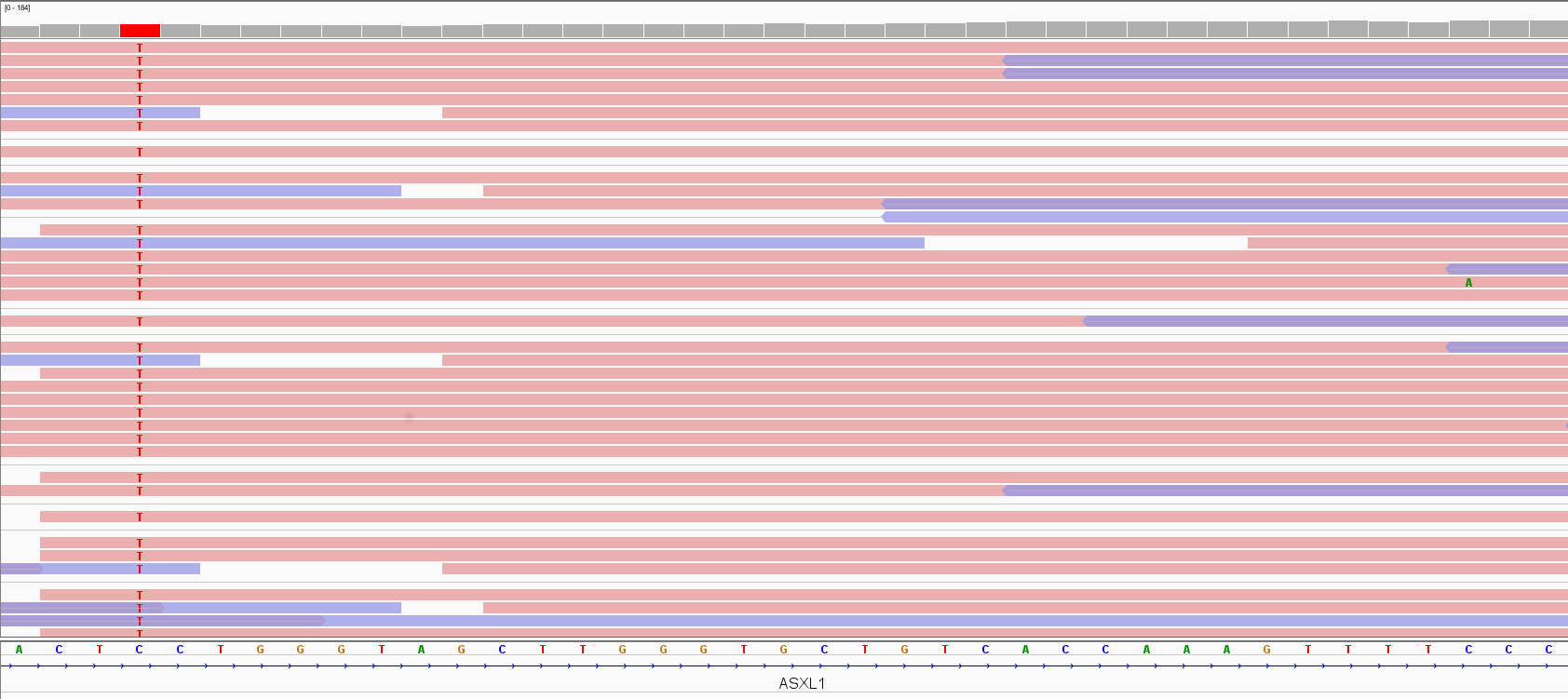
Figure 5. Variant visualization by IGV

---

The GATK variant calling pipeline first produces a genomic VCF (gVCF), whose main difference with VCF is that it records all sites in a target whether there is a variant or not, while VCF contains only information for variant sites, preparing multiple samples for joint genotyping and creation of a multi-sample VCF whose variants can undergo quality filtering in order to obtain the final set of quality-curated variants ready to be annotated.

In downstream analyses, annotations can be added to VCF files themselves or information in VCF files can be either annotated in TAB- or comma- deimited files to be visually inspected for clinical variant searching or used as input to prioritization programs.

Requirements

This tutorial is based on the Galaxy platform, therefore a basic knowledge of Galaxy is required to get most out of the course. In particular, we’ll use the European Galaxy server running at https://usegalaxy.eu.

Registration is free, and you get access to 250GB of disk space for your analysis.

1. Open your browser. We recommend Chrome or Firefox (please don’t use Internet Explorer or Safari).
2. Go to https://usegalaxy.eu
   • If you have previously registered on this server just log in:
     • On the top menu select: User -> Login
     • Enter your user/password
     • Click Submit
   • If you haven’t registered on this server, you’ll need to do now.
     • On the top menu select: User -> Register
     • Enter your email, choose a password, repeat it and add a one word name (lower case)
     • Click Submit

To familiarize with the Galaxy interface (e.g. working with histories, importing dataset), we suggest to follow the Galaxy 101 tutorial.

Datasets

Input datasets used in this course are available:

• at Zenodo, an open-access repository developed under the European OpenAIRE program and operated by CERN
• as Shared Data Libraries in Galaxy: Galaxy courses / Sigu

Use cases

We selected some case studies for this tutorial. We suggest you to start with a simple case (e.g. Fam A) for the first run of the tutorial, and repeat it with the more complex ones. At the end of the page you will be able to compare your candidate variants with the list of true pathogenic variants.

Family	Proband	Father	Mother	Description	HPO	Reference
Fam A	FamilyA_P	FamilyX_F	FamilyX_M	Five-year-old female patiant; Short stature; Severe intellectual disability; Seizures; Polymicrogyria; Cerebellar hemisphere hypoplasia; Postnatal microcephaly; Microphthalmia; Optic nerve coloboma; Malformation of the heart and great vessels; Intestinal malrotation; Hydronephrosis; Cryptorchidism	HP:0004322, HP:0010864, HP:0001250, HP:0002126, HP:0100307, HP:0005484, HP:0000568, HP:0000588, HP:0001627, HP:0030962, HP:0002566, HP:0000126, HP:0000028	hg38
Fam B	FamilyB_P	FamilyB_F	FamilyB_M	Four-year-old male patient; Intellectual disability; Malformation of the heart and great vessels; Abnormality of blood and blood-forming tissues; Short Stature; Velopharyngeal insufficiency; Coarse facial features with high, narrow forehead, shallow orbits, depressed nasal bridge, anteverted nares, long philtrum, flat face, and macroglossia	HP:0001249, HP:0001627, HP:0030962, HP:0001871, HP:0004322, HP:0000220, HP:0000280, HP:0000341, HP:0000348, HP:0000586, HP:0005280, HP:0000463, HP:0000343, HP:0012368, HP:0000158	hg38
Fam C	FamilyC_P	FamilyC_F	FamilyC_M	Eighteen-year-old female patient; Non-consanguineous Caucasian parents; Unremarkable family history; Normal intellectual development; Born at term by normal delivery; Oligohydramnios; Decreased fetal movements; Distal arthrogryposis; Cutaneous finger syndactyly; Scoliosis; Popliteal pterygium; Recurrent pneumonia; Restrictive ventilatory defect; Skeletal muscle atrophy	HP:0001562, HP:0001558, HP:0005684, HP:0010554, HP:0002650, HP:0009756, HP:0006532, HP:0002091, HP:0003202	hg38
Fam D	FamilyD_P	FamilyD_F	FamilyX_M	Ten-year-old male patient; Non-consanguineous Caucasian parents; Unremarkable family history; Severe intellectual disability; Absent speech; Seizure; Ataxia; Stereotypy; Sudden episodic apnea; Postnatal microcephaly; Hypoplasia of the corpus callosum; Strabismus; Myopia; Constipation; Single transverse palmar crease; Narrow forehead; Wide nasal bridge; Short philtrum; Full cheeks; Wide mouth; Thickened helices	HP:0010864, HP:0001344, HP:0001250, HP:0001251, HP:0000733, HP:0002882, HP:0005484, HP:0002079, HP:0000486, HP:0000545, HP:0002019, HP:0000954, HP:0000341, HP:0000431, HP:0000322, HP:0000293, HP:0000154, HP:0000391	hg38
Fam E	FamilyE_P	FamilyX_F	FamilyE_M	Thirty-year-old woman. Three consecutive pregnancy terminations due to fetal malformations, Woman phenotype included: High forehead, Hypertelorism, Mandibular prognathia. Fetal malformations observed: Cystic hygroma, Cerebellar agenesis, Hypoplastic nasal bone, Cleft lip , Bilateral hydronephrosis, Renal hypertrophy, Hypoplasia of external genitalia, Hypertrophic cardiomyopathy, Ventricular septal defect, Omphalocele	HP:0000348, HP:0000316, HP:0000303, HP:0000476, HP:0012642, HP:0011430, HP:0410030, HP:0000126, HP:0000811, HP:0001639, HP:0001629, HP:0001539	hg38

Get data

hands_on Hands-on: Data upload

1. Create a new history for this tutorial and give it a meaningful name (e.g. Clinical genomics)

   tip Tip: Creating a new history

   Click the new-history icon at the top of the history panel

   If the new-history is missing:

   1. Click on the galaxy-gear icon (History options) on the top of the history panel
   2. Select the option Create New from the menu

   tip Tip: Renaming a history

   1. Click on Unnamed history (or the current name of the history) (Click to rename history) at the top of your history panel
   2. Type the new name
   3. Press Enter

2. Files are available on the Galaxy server through a Shared Data Libraries in Galaxy courses/Sigu. This is the preferred solution as you will save time and disk space.

   tip Tip: Importing data from a data library

   As an alternative to uploading the data from a URL or your computer, the files may also have been made available from a shared data library:

   • Go into Shared data (top panel) then Data libraries

   • Find the correct folder (ask your instructor)

   • Select the desired files
   • Click on the To History button near the top and select as Datasets from the dropdown menu
   • In the pop-up window, select the history you want to import the files to (or create a new one)
   • Click on Import

   The same files are available at Zenodo (1, 2, 3):

   FASTQ reads:

   https://zenodo.org/record/3531578/files/HighQuality_Reads.fastq.gz
   https://zenodo.org/record/3531578/files/LowQuality_Reads.fastq.gz
   

   Family A:

   https://zenodo.org/record/3531578/files/FamilyA_P.bam
   

   Family B:

   https://zenodo.org/record/nnnnnnn/files/FamilyB_P.bam
   https://zenodo.org/record/3531578/files/FamilyB_F.bam
   https://zenodo.org/record/3531578/files/FamilyB_M.bam
   

   Family C:

   https://zenodo.org/record/nnnnnnn/files/FamilyC_P.bam
   https://zenodo.org/record/4264088/files/FamilyC_F.bam
   https://zenodo.org/record/4264088/files/FamilyC_M.bam
   

   Family D:

   https://zenodo.org/record/4197066/files/FamilyD_P.bam
   https://zenodo.org/record/4197066/files/FamilyD_F.bam
   

   Family E:

   https://zenodo.org/record/nnnnnnn/files/FamilyE_P.bam
   https://zenodo.org/record/3531578/files/FamilyE_M.bam
   

   Files shared across families:

   https://zenodo.org/record/4197066/files/FamilyX_M.bam
   https://zenodo.org/record/4264088/files/FamilyX_F.bam
   

   tip Tip: Importing data via links

   • Copy the link location

   • Open the Galaxy Upload Manager (galaxy-upload on the top-right of the tool panel)

   • Select Paste/Fetch Data

   • Paste the link into the text field

   • Press Start

   • Close the window

   By default, Galaxy uses the URL as the name, so rename the files with a more useful name.

   comment Note

   All the files are based on hg38 reference genome which is available with pre-built indexes for widely used tools such as bwa-mem and samtools by selecting hg38 version as an option under “(Using) reference genome”).

3. In case you import datasets from Zenodo, check that all datasets in your history have their datatypes assigned correctly, and fix it when necessary. For example, to assign BED datatype do the following:

   tip Tip: Changing the datatype

   • Click on the galaxy-pencil pencil icon for the dataset to edit its attributes
   • In the central panel, click on the galaxy-chart-select-data Datatypes tab on the top
   • Select bed
   • Click the Change datatype button

4. Rename the datasets

   For datasets uploaded via a link, Galaxy will use the link as the dataset name. In this case you may rename datasets.

   tip Tip: Renaming a dataset

   • Click on the galaxy-pencil pencil icon for the dataset to edit its attributes
   • In the central panel, change the Name field
   • Click the Save button

Quality control

In-depth quality control (QC) of data generated during an NGS experiment is crucial for an accurate interpretation of the results. For example an accurate QC could help in identifying poor quality experiments, sequence contamination or genomic regions with low sequence coverage, and all these factors have a large impact on the downstream processing.

Most of the programs used during an NSG workflow do not include steps for quality control, therefore artifacts needs to be detected using ad-hod developed tools for QC. The table summarizes the main tools available at https://usegalaxy.eu for quality checking, at each step of the analysis.

NGS workflow step	File format	Tools for quality control
Sample to reads	fastQ	FastQC
Reads to alignments	BAM	General statistics: bam.io.bio, samtools; target coverage: Picard CollectHSMetrics; per base coverage depth: bedtools
Alignments to variants	VCF	vcf.io.bio

---

Quality control of FASTQ files

Before starting the analysis workflow, you should identify possible issues that could affect alignment and variant calling. This first step of quality control is based on the raw sequence data (fastQ) generated by the sequencer. Common issues with sequence quality can be easily addressed by further processing your original sequences to trim or remove low-quality reads. In presence of severe artefacts you should consider to repeat the experiment instead of starting the downstream analysis that will generate poor quality results, according to the rule ‘garbage in, garbage out’.

Here we’ll use the FastQC software for a standard quality check, using the two FASTQ files HighQuality_Reads.fastq and LowQuality_Reads.fastq.

FastQC is relatively easy to use. The output of FastQC consists of multiple modules analysing a specific aspect of the quality of the data. A detailed help can be found in the help manual.

The names of the modules are preceded by an icon that reflects the quality of the data, and indicates whether the results of the module are:

• normal (green)
• slightly abnormal (orange)
• very unusual (red)

comment Note on FastQC interpretation

These evaluations must be taken in the context of what you are expecting from your dataset. For FastQC a normal sample includes random sequences with high diversity. If your experiment generates biased libraries (e.g. low complexity libraries) you should interpret the report with attention. In general, you should concentrate on the icons different from green and try to understand the reasons for this behaviour.

hands_on Hands-on: Computing sequence quality with FastQC

1. Run FastQC tool on your fastq datasets HighQuality_Reads.fastq and LowQuality_Reads.fastq. You can select both datasets with the Multiple datasets option.

   tip Tip: Select multiple datasets

   1. Click on param-files Multiple datasets
   2. Select several files by keeping the Ctrl (or COMMAND) key pressed and clicking on the files of interest

   For each input file you will get two datasets, one with the raw QC statistics and another with an HTML report with figures.

2. Using the MultiQC tool software, you can aggregate multiple raw FastQC output in one unique report. This helps in comparing multiple samples at the same time in order to quickly identify low quality samples that will be displayed as outliers.
   • “Which tool was used generate logs?”: FastQC
     • In “FastQC output”
       • “Type of FastQC output?”: Raw data
       • param-files “FastQC output”: the two RawData outputs of FastQC tool
3. Inspect MultiQC report

For a detailed explanation of the different analysis modules of FastQC you may refer to the Quality control tutorial.

question Questions

1. Based on the MultiQC report, check which modules highlight differences in sequence quality betwen the two datasets

Quality control of BAM files

Fast quality check with bam.iobio.io

BAM files are binary files containing information on the sequences aligned onto a reference genome. Exploring BAM files you can address several questions, e.g.:

• which is the amount of duplicated sequences? For non PCR-free protocols, it should be < 15%. Duplicated sequences are not used in downstream analysis to identify variants, therefore should be kept at a minimum to avoid waste of reagents.
• which is the fraction of unmapped reads? It should be < 2%. If higher, you should ask why so many reads are not properly mapped onto the reference genome. One possible reason could be sample contamination.

In Galaxy, BAM files can be explored using the bam.iobio.io web app. Leveraging on random subsampling of reads, bam.iobio.io quickly draws several quality control reports (Figure 6).

On top of each plot, clicking on the question mark you can open a window with a detailed explanation of the expected output. The number of reads sampled is shown at the top-right of the page, and can be increased by clicking on the arrow.

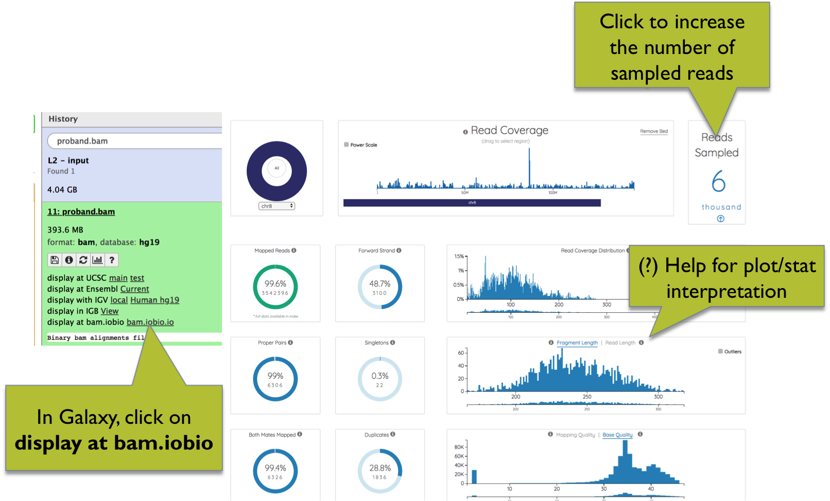
Figure 6. BAM quality control using bam.iobio.io

hands_on Hands-on: Computing BAM quality with bam.iobio.io

1. Run bam.iobio.io tool on a BAM dataset. To start bam.iobio.io click on the link diplay at bam.iobio.io in the dataset section. Please note that the link will be visible only for datasets with the appropriate database field set to hg38

   tip Tip: Changing Database/Build (dbkey)

   • Click on the galaxy-pencil pencil icon for the dataset to edit its attributes
   • In the central panel, change the Database/Build field
   • Select your desired database key from the dropdown list: hg38
   • Click the Save button

   question Questions

   1. Which is the amount of duplicated sequences?
   2. And the fraction of aligned reads?

Coverage metrics with Picard

Collect Hybrid Selection (HS) Metrics tool tool computes a set of metrics that are specific for sequence datasets generated through hybrid-selection, a commonly used protocol to capture specific sequences for targeted experiments such as panels and exome sequencing.

In order to run this tool you need a file with the aligned sequences in BAM format, and files with the intervals corresponding to bait and target regions. These files can be generally obtained from the website of the kit manufacturer.

comment Note

Please note that interval files are generally available as BED files, and must be converted in Picard interval_list format using Picard’s BedToInterval tool before running CollectHsMetrics - see the hands on below for details.

Metrics generated by CollectHsMetrics are grouped into three classes:

• Basic sequencing metrics: genome size, the number of reads, the number of aligned reads, the number of unique reads, etc.
• Metrics for evaluating the performance of the wet-lab protocol: number of bases mapping on/off/near baits, number of bases mapping on target, etc.
• Metrics for coverage estimation: mean bait coverage, mean and median target coverage, the percentage of bases covered at different coverage (e.g. 1X, 2X, 10X, 20X, …), the percentage of filtered bases, etc.

For a detailed description of the output see Picard’s CollectHsMetrics

In the next tutorial we will compute hybrid-selection metrics for BAM files containing aligned sequences from an exome sequencing experiment.

hands_on Hands-on: Computing BAM statistics with Picard CollectHsMetrics

1. Before computing the statistics, we first need to convert the BED files with bait and target regions, in Picard interval_list format. Remember that you can select multiple datasets with the Multiple datasets option.

   tip Tip: Select multiple datasets

   1. Click on param-files Multiple datasets
   2. Select several files by keeping the Ctrl (or COMMAND) key pressed and clicking on the files of interest

   Run BedToIntervalList tool to convert BED files.

   • “Load picard dictionary file from?”: Local cache
     • In “Use dictionary from the list”: Human (Homo sapiens): hg38
   • “Select coordinate dataset or dataset collection?”: your BED file to be converted

2. Run CollectHsMetrics tool using as input the BAM files and the intervals in Picard interval_list format, corresponding to the bait and target regions, generated in the previous step.

3. Use MultiQC tool to aggregate CollectHsMetrics output in one unique report to facilitate the comparison across multiple samples.
   • “Which tool was used generate logs?”: Picard
     • In “Picard output”
       • “Type of Picard output?”: HS Metrics
       • param-files “Picard output”: the output of CollectHsMetrics tool

4. Inspect MultiQC tool report

   question Questions

   1. Which is the average target coverage?
   2. And the fraction of bases covered at least 10X?

Variant annotation

After the generation of a high-quality set of mapped read pairs, we can proceed to call different classes of DNA variants. Users interested in germline variant calling can refer to related Galaxy’s tutorials, e.g. Exome sequencing data analysis for diagnosing a genetic disease.

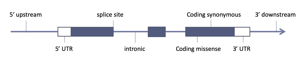
Variant callers usually provide us with a simple list of sequence variants (genomic coordinates + reference and variant alleles) plus genotypes and genotype-likelihoods. Variant annotation is the process of adding informations to these variants using multiple sources (e.g. public databases). We are usually interested in knowing for example if a specific variant overlaps with a gene, if it falls into an exon of that gene, if it’s a coding exon, what type of change the variant causes to the encoded amino acid (missense, nonsense, frameshift), etc.

---

Gene model

The choice of gene model is essential for variant downstream variant annotation: it describe genomic positions of genes and each exon-intron exact locations

Different gene models can give different annotations:

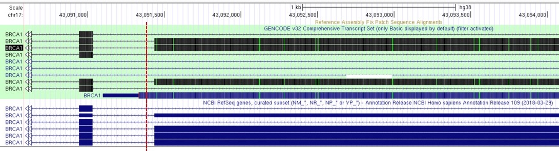
Figure 1. Variant indicated by the red dashed line can be annotated as intronic or exonic (on one of the UCSC transcript variants), depending on the adopted gene model:

Source	Description
RefSeq	A comprehensive, integrated, non-redundant, well-annotated set of reference sequences including genomic, transcript, and protein
Ensembl	Integrates and distributes reference datasets and analysis tools. Based at EMBL-EBI
Gencode	A project to identify and classify all gene features in the human and mouse genomes with high accuracy based on biological evidence. Based on the ENCODE consortium

---

Sequence variant nomenclature

Variant nomenclature should be described univocally:

Source	Description
HGVS	HGVS-nomenclature serves as an international standard for the description of DNA, RNA and protein sequence variants
HGMC	HUGO Gene Nomenclature Committee is responsible for approving unique symbols and names for human loci, including protein coding genes, ncRNA genes and pseudogenes, to allow unambiguous scientific communication

Variant class

Sequence features used in biological sequence annotation should be defined using the Sequence Ontology, a collaborative project for the definition of sequence features used in biological sequence annotation.

Among the main sources of variant annotation are:

Population sequencing db

• gnomAD
• ExAC
• 1000 Genomes Project
• NHLBI-ESP 6500 exomes
• dbSNP

Variant-disease/gene-disease db

• Human Gene Mutation Database
• clinically relevant variants known in a gene
• Simple ClinVar
• Online Mendelian Inheritance in Man
• dbNSFP, a big database of curated annotations and precomputed functional predictions for all potential non-synonymous and splice-site single-nucleotide variants in the human genome

Several tools and softwares are available for variant annotation, here is a list of the most used ones:

Annotation Software and tools

Local installation:

• Variant Effect Predictor
• ANNOVAR
• Single Nucleotide Polymorphism Effect
• KGGSeq

Web interface:

• wAnnovar
• VEP

---

Annotation and filtering with SnpEFF

For variant annotations we’ll use SnpEff, a software for genomic variant annotation and functional effect prediction.

hands_on Hands-on: Variant annotations with SnpEff

1. Choose SnpEff eff tool (“annotate variants”, not “annotate variants for SARS-CoV-2”)
   • param-file “Sequence changes (SNPs, MNPs, InDels)”: the uploaded VCF file
   • “Input format”: VCF
   • “Output format”: VCF (only if input is VCF)
   • “Genome source”: Locally installed snpEff database
     • “Genome”: Homo sapiens: hg38 (or a similarly named option)
   • “Produce Summary Stats”: Yes

   tip Tip: Annotation options

   You can Select/Unselect many Annotation options checking from the list (i.e “Use gene ID instead of gene name (VCF output)” or “Only use canonical transcripts”)

   tip Tip: Filter output

   You can narrow down the output list of annotated variants, filtering out specific types of changes, choosing from the five choices shown in the Filter output menu (i.e “Do not show DOWNSTREAM changes” or “Do not show INTERGENIC changes”)or selecting “Yes” from Filter out specific Effects and selecting from all the type of possible categories

Two output file will be created:

1. a Summary Stats HTML report, with general metrics such as the distribution of variants across gene features;
2. a VCF file with annotations of variant effects added to the INFO column.

Variant prioritization

Once annotated, variants need to be filtered and prioritized. The number of variants returned by genomic sequencing varies from tens of thousands (WES) to millions (WGS).

No universal filters are available, they depend on the experimental features

Variant impact

First of all you usually want to filter variants by consequence on the encoded protein, keeping those which have an higher impact on protein:

• Missense
• Nonsense
• Splice sites
• Frameshift indels
• Inframe indels

Variant frequency

• Common variants are unlikely associated with a clinical condition
• A rare variant will probably have a higher functional effect on the protein
• Frequency cut-off have to be customized on each different case
• Typical cut-offs: 1% - 0.1%
• Allele frequencies may differ a lot between different populations

Variant effect prediction Tools

• Tools that predict consequences of amino acid substitutions on protein function

• They give a score and/or a prediction in terms of “Tolerated”, “Deleterious” (SIFT) or “Probably Damaging”, “Possibly Damaging”, “Benign” (Polyphen2)

  • fitCons
  • GERP++
  • SIFT
  • PolyPhen2
  • CADD
  • DANN
  • Condel
  • fathmm
  • MutationTaster
  • MutationAssessor
  • REVEL

ACMG/AMP 2015 guidelines

The American College of Medical Genetics and the Association for Molecular Pathology published guidelines for the interpretation of sequence variants in May of 2015 (Richards S. et al, 2015). This report describes updated standards and guidelines for classifying sequence variants by using criteria informed by expert opinion and experience

• 28 evaluation criteria for the clinical interpretation of variants. Criteria falls into 3 sets:
  • pathogenic/likely pathogenic (P/LP)
  • benign/likely benign (B/LB)
  • variant of unknown significance (VUS)
• Intervar: software for automatical interpretation of the 28 criteria. Two major steps:
• automatical interpretation by 28 criteria
• manual adjustment to re-interpret the clinical significance

Prioritization

Phenotype-based prioritization tools are methods working by comparing the phenotypes of a patient with gene-phenotype known associations.

• Phenolyzer: Phenotype Based Gene Analyzer, a tool to prioritize genes based on user-specific disease/phenotype terms

hands_on Hands-on: Variant prioritization

Using knowledge gained on Genomic databases and variant annotation section, try to annotate, filter and prioritize an example exome variant data, using two disease terms

• Download a VCF file from the dataset, as learned in the Home section

• Go to wANNOVAR

• Use the vcf file as input file and hearing loss and deafness autosomal recessive, as disease terms to prioritize results

• Choose rare recessive Mendelian disease as Disease Model in the Parameter Settings section

• Provide an istitutional email address and submit the Job

• … wait for results …

  In the results page you can navigate and download results. Click Show in the Network Visualization section to see Phenolyzer prioritization results

GEMINI for variant filtering

Now, we’ll use the VCF file annotated with SnpEff to filter variants considering the relationship between family members. For this purpose we’ll use GEMINI, a framework including different modules for analysis of human variants. First, we need to inform GEMINI about the relationship between the samples and their phenotypes (affected vs not affected). This information is stored in a pedigree file in PED format. In next Hands-on you’ll learn how to manually generate a pedigree file.

hands_on Hands-on: Creating a GEMINI pedigree file

1. Create an example PED-formatted pedigree file for a trio:

   #family_id    name        paternal_id    maternal_id    sex    phenotype
   Fam_A         father_ID   0              0              1      1
   Fam_A         mother_ID   0              0              2      1
   Fam_A         proband_ID  father_ID      mother_ID      1      2
   

   and set its datatype to tabular.

   tip Tip: Creating a new file

   • Open the Galaxy Upload Manager
   • Select Paste/Fetch Data

   • Paste the file contents into the text field

   • Change Type from “Auto-detect” to tabular

   • Press Start and Close the window

   warning Remember those sample names

   Names in the pedigree file should match the sample names in your VCF file in order to be recongnized by GEMINI. If names are different, samples will not be recognized and therefore you will not be able to filter variants by patterns of genetic inheritance.

   details More on PED files

   The PED format is explained in the help section of GEMINI load tool and here

   Take a moment and try to understand the information that is encoded in the PED dataset we are using here.

Next, in order to formulate queries to extract variants matching your selection criteria, variants and their annotations need to be stored in a format accepted by GEMINI. This task is accomplished by the GEMINI load tool, which accepts as input your SnpEFF SnpEff annotated VCF file together with the pedigree file.

hands_on Hands-on: Creating a GEMINI database

1. GEMINI load tool with
   • param-file “VCF dataset to be loaded in the GEMINI database”: the output of SnpEff eff tool
   • “The variants in this input are”: annotated with snpEff

   • “This input comes with genotype calls for its samples”: Yes

     Our examples VCf include genotype calls.

   • “Choose a gemini annotation source”: select the latest available annotations snapshot (most likely, there will be only one)
   • “Sample and family information in PED format”: the pedigree file prepared above
   • “Load the following optional content into the database”
     • param-check “GERP scores”
     • param-check “CADD scores”
     • param-check “Gene tables”
     • param-check “Sample genotypes”
     • param-check “variant INFO field”

     Checked the following:

     • “only variants that passed all filters”

       This retains only high quality variants, e.g variants with the value in the FILTER column equals to PASS

     Leave unchecked the following:

     • “Genotype likelihoods (sample PLs)”

       Our VCFs does not contain these values

This generates a GEMINI-specific dataset, which can only be processed with other GEMINI tools. In fact, every analysis with a GEMINI tool starts with the GEMINI database obtained by GEMINI load tool.

details The GEMINI suite of tools

The GEMINI framework is composed by a large number of utilities.

The Somatic variant calling tutorial demonstrates the use of the GEMINI annotate and GEMINI query tools, and tries to introduce some essential bits of GEMINI’s SQL-like syntax.

For a thorough explanation of all GEMINI tools and functionality visit the GEMINI documentation.

Candidate variant detection

Here you’ll learn how to use GEMINI inheritance pattern tool to report all variants fitting any specific inheritance model. You’ll be able to select any of the following inheritance patterns:

• Autosomal recessive
• Autosomal dominant
• X-linked recessive
• X-linked dominant
• Autosomal de-novo
• X-linked de-novo
• Compound heterozygous
• Loss of heterozygosity (LOH) events

Below is how you can perform the query for inherited autosomal recessive variants. Feel free to run analogous queries for other types of variants that you think could plausibly be causative for your case study.

hands_on Hands-on: Filtering variants by inheritance pattern

1. GEMINI inheritance pattern tool
   • “GEMINI database”: the GEMINI database of annotated variants; output of GEMINI load tool
   • “Your assumption about the inheritance pattern of the phenotype of interest”: e.g. Autosomal recessive
     • param-repeat “Additional constraints on variants”

       • “Additional constraints expressed in SQL syntax”: impact_severity != 'LOW'

         This will remove variants with low impact severity (i.e., silent mutations and variants outside coding regions). Leave this box empty to report all variants independently of their impact.

     • “Include hits with less convincing inheritance patterns”: No

       Account for errors in phenotype assignment - meaningful for large families

     • “Report candidates shared by unaffected samples”: No

       Account for incomplete penetrance - meaningful for large families

   • “Family-wise criteria for variant selection”: keep default settings

     This section is not useful when you have data from just one family.

   • In “Output - included information”
     • “Set of columns to include in the variant report table”: Custom (report user-specified columns)
       • “Choose columns to include in the report”:
         • param-check “alternative allele frequency (max_aaf_all)”
       • “Additional columns (comma-separated)”: chrom, start, ref, alt, impact, gene, clinvar_sig, clinvar_disease_name, clinvar_gene_phenotype, rs_ids

   details ClinVar annotations

   clinvar_sig and clinvar_disease_name annotations refer to the particular variant, clinvar_gene_phenotype provides information about the gene harbouring the variant.

question Question

From the output of GEMINI inheritance pattern, can you identify the most likely candidate variant?

details More GEMINI usage examples

While only demonstrating command line use of GEMINI, the following tutorial slides may give you additional ideas for variant queries and filters:

• Introduction to GEMINI
• Identifying de novo mutations with GEMINI
• Identifying recessive gene candidates with GEMINI
• Identifying dominant gene candidates with GEMINI

Solutions

Below you will find the true patogenic variants for all the case studies.

solution Solutions

• Family A: WDR37, FIXME-VARIANT, de novo
• Family B: GNAPTB, FIXME-VARIANT, compound heterozigosity
• Family C: ECEL1, FIXME-VARIANT, compound heterozigosity
• Family D: TCF4, FIXME-VARIANT, parental mosaicism
• Family E: GPC3, FIXME-VARIANT, X-linked

Advanced analysis

To address in more details quality control strategies, structural variants analysis (i.e. CNVs), or identification of RoHs you can move forward to the Advanced tutorial.

Contributors

• Tommaso Pippucci - Sant’Orsola-Malpighi University Hospital, Bologna, Italy
• Alessandro Bruselles - Istituto Superiore di Sanità, Rome, Italy
• Andrea Ciolfi - Ospedale Pediatrico Bambino Gesù, IRCCS, Rome, Italy
• Gianmauro Cuccuru - Albert Ludwigs University, Freiburg, Germany
• Giuseppe Marangi - Institute of Genomic Medicine, Fondazione Policlinico Universitario A. Gemelli IRCCS, Università Cattolica del Sacro Cuore, Roma, Italy
• Paolo Uva - IRCCS G. Gaslini, Genoa, Italy

Citing this Tutorial

1. Alessandro Bruselles, Andrea Ciolfi, Gianmauro Cuccuru, Giuseppe Marangi, Paolo Uva, Tommaso Pippucci, 2020 Data analysis and interpretation for clinical genomics (Galaxy Training Materials). /clinical_genomics/ Online; accessed TODAY
2. Batut et al., 2018 Community-Driven Data Analysis Training for Biology Cell Systems 10.1016/j.cels.2018.05.012

details BibTeX

@misc{-,
    author = "Alessandro Bruselles and Andrea Ciolfi and Gianmauro Cuccuru and Giuseppe Marangi and Paolo Uva and Tommaso Pippucci",
    title = "Data analysis and interpretation for clinical genomics (Galaxy Training Materials)",
    year = "2020",
    month = "10",
    day = "21"
    url = "\url{/clinical_genomics/}",
    note = "[Online; accessed TODAY]"
}
@article{Batut_2018,
        doi = {10.1016/j.cels.2018.05.012},
        url = {https://doi.org/10.1016%2Fj.cels.2018.05.012},
        year = 2018,
        month = {jun},
        publisher = {Elsevier {BV}},
        volume = {6},
        number = {6},
        pages = {752--758.e1},
        author = {B{\'{e}}r{\'{e}}nice Batut and Saskia Hiltemann and Andrea Bagnacani and Dannon Baker and Vivek Bhardwaj and Clemens Blank and Anthony Bretaudeau and Loraine Brillet-Gu{\'{e}}guen and Martin {\v{C}}ech and John Chilton and Dave Clements and Olivia Doppelt-Azeroual and Anika Erxleben and Mallory Ann Freeberg and Simon Gladman and Youri Hoogstrate and Hans-Rudolf Hotz and Torsten Houwaart and Pratik Jagtap and Delphine Larivi{\`{e}}re and Gildas Le Corguill{\'{e}} and Thomas Manke and Fabien Mareuil and Fidel Ram{\'{\i}}rez and Devon Ryan and Florian Christoph Sigloch and Nicola Soranzo and Joachim Wolff and Pavankumar Videm and Markus Wolfien and Aisanjiang Wubuli and Dilmurat Yusuf and James Taylor and Rolf Backofen and Anton Nekrutenko and Björn Grüning},
        title = {Community-Driven Data Analysis Training for Biology},
        journal = {Cell Systems}
}