Advanced data analysis of genomic data
 Alessandro Bruselles,
  Andrea Ciolfi,
  Gianmauro Cuccuru,
  Giuseppe Marangi,
  Paolo Uva,
  Tommaso Pippucci
Overview
question Questionsobjectives Objectives
What is the minimal depth of coverage of target regions in a typical clinical genomics setting?
Which are the most common computational strategies to identify copy-number alterations in NGS experiments?
To calculate sequencing statistics
To manipulate genomic regions files
To identify genomic mosaic variants
To use webtools for genomic variants annotation
To analyze CNV and Regions of Homozygosity (ROH)
time Time estimation: 2 hours
last_modification Last modification: Oct 23, 2020
Introduction
This section of the tutorial will cover in more details many different aspects of data analysis and interpretation for clinical genomics. It will delve into quality control procedures, and into specific strategies to be used to identify different variations of individuals’ genetic architecture, as mosaic variants, copy number variants, and regions of homozygosity.
Agenda
In this tutorial, we will cover:
Requirements
This tutorial requires that the basic course has been completed successfully or that the user is familiar with the Galaxy platform. In particular, we’ll use the European Galaxy server running at https://usegalaxy.eu.
Datasets
Input datasets are available:
- at Zenodo, an open-access repository developed under the European OpenAIRE program and operated by CERN
- as Shared Data Libraries in Galaxy: Galaxy courses / Sigu
Quality control
Computation of per-base coverage depth at specific genomic intervals
Commercial next-generation sequencing platforms usually provide users with analysis programs, which include tools for the identification of low coverage regions (for instance, target regions that have a coverage depth lower than 20x).
The present tutorial is aimed to show how to perform a custom coverage analysis of NGS experiments by using tools that are available in Galaxy.
Starting material:
- Alignment (bam) file(s) on which you want to perform the coverage evaluation.
- A reference bed file listing the genomic regions for which you want to obtain coverage data. If you performed a targeted sequencing experiment by using commercial kits (either custom or from the catalogue), you should already have obtained a bed file listing the target regions: it should be the file you want to use.
comment BED format specifications
BED files are tab-delimited files with one line for each genomic region. The first 3 fields (columns) are required:
- chromosome
- the starting position
- the ending position
Further columns may be present but are optional. Additional details may be found here: UCSC BED format specifications
Please be aware that in BED files the description of genomic regions follows the “0-start, half-open” coordinate system. Further details may be found here: the “0-based, half-open” UCSC Genome Browser Coordinate Counting Systems. Practically speaking, it means that the starting position is diminished by 1 bp with respect to the actual position. For instance, the region “chr2 50149071 50149399” in a bed file corresponds to the genomic interval from position 50149072 (included) to position 50149399 (included) on chromosome 2 (when the first base of the chromosome is defined as position 1). If you want to indicate a single base position in a bed file, it should be written like this: “chr2 50149071 50149072” .
hands_on Hands-on: Compute per base coverage depth with BEDtools
Before starting, you have to upload the files you need for the analysis, following standard Galaxy procedure.
You may use files provided as examples with this tutorial and called
Panel_alignment.bamandPanel_Target_regions.bed.Please check that uploaded file datatypes (formats) are properly recognized by selecting
edit attributes(i.e. the pencil sign in correspondence of each file you can find in your history) (indicated by the red arrow in figure 1) and then the tab datatypes (the blue arrow in figure 1). If the datatype is wrong, select the correct one from the drop-down list and press thechange datatypebutton (the green arrow in figure 1).
Figure 1
Once ready, you can select the tool named
bedtools Compute both the depth and
   breadth of coverage
in theOperate on Genomic Intervalssection (see the red arrow in figure 2).
- Select the bed file listing the target regions as “file A” (blue arrow in figure 2) and the bam file(s) you want to analyze as “file B” (green arrow in figure 2) (they should be listed in the drop-down menu if they have the correct format). You may analyze one or more bam files in a single run.
- If you want to analyze two or more .bam files, you can further choose if you want all the results in a single file or one output file per input “file B” by selecting the desired option under the
Combined or separate output filesmenu.- Select “Yes” for the option
Report the depth at each position in each A feature(yellow arrow in figure 2) and check that all the other options are set to “No”.Star (Execute) the analysis.
Figure 2
Output file, which will be called “coverage_depth.bed” from now on, will contain all the fields of the original target_regions.bed file plus two further columns:
- the first value indicates a specific base within the reported genomic interval. For instance, if the genomic interval described by the first 3 field is “chr2 50149071 50149072” and the first new field reports the number 1000, it means that the coverage value refers to nucleotide 50150071 (i.e.: 50149071 + 1000) on chromosome 2;
- the second value indicates the depth of coverage for the defined base.
hands_on Hands-on: Sort files
Since entries in the “coverage_depth.bed” may not be in the desired order, you can sort it by genomic positions. For this purpose you may want to use the
Sorttool in theText Manipulationsection (check out the blue arrow in figure 3).You may sequentially sort on different columns:
- first you can sort by chromosome by selecting column 1 (green arrow in figure 3) in “ascending order” and selecting the “flavor”
Natural/Version sort (-V), which allows for sorting chromosomes in their “natural” order (with alphabetical order chr10 will be right after chr1, chr2 after chr19 and so on);- after inserting a new column section (red arrow in figure 3), you can sort by column 2 in “ascending order” with
Fast numeric sort (-n);- after inserting a further column section, you can sort by column 3 in “ascending order” with
Fast numeric sort (-n);- after inserting a final column section, you can sort by column 3 in “ascending order” with
Fast numeric sort (-n).
Figure 3
The obtained output file, which will be called “sorted_coverage_depth.bed” from now on, will be sorted first by chromosome, then by starting position, by ending position and by the actual position of the specific base in the considered genomic interval.
hands_on Hands-on: Remove duplicate rows
If your file contains duplicated lines you may want to remove them for further processing. For this purpose you can use the
Unique lines assuming sorted input filetool in theText Manipulationsection.
hands_on Hands-on: Some manipulation of the bed file
You may follow the following steps to manipulate the “sorted_coverage_depth.bed” and to obtain a bed file listing the exact base position to which each coverage value is referred. For instance instead of having “chr2 50149071 50149399 NRXN1 1 2335” in the first row of your file, you will get “chr2 50149071 50149072 NRXN1 2335”.
These steps will add further columns at the end of each line defining the base position with the “0-start, half-open” coordinate system.
- Select the
Compute an expression on every rowtool in theText Manipulationsection (indicated by the blue arrow in figure 4);- add the following expression “c2+c5-1” to obtain the sum of the values in columns 2 and 5 minus 1 (it will be used as the new starting position in the final file);
- select the file “sorted_coverage_depth.bed”;
- select “yes” to
round Results?(green arrow in figure 4);- execute;
- you can rename the output as “temp1_coverage_depth.bed”;
- select the
Compute an expression on every rowtool in theText Manipulationsection;- add the following expression “c2+c5” to obtain the sum of the values in columns 2 and 5 (it will be used as the new ending position in the final file). You can also use the expression ;
- select the file “temp1_coverage_depth.bed”;
- select “yes” to
round Results?;- execute;
- you can rename the output as “temp2_coverage_depth.bed”;
- select the
Table Computetool in theText Manipulationsection (indicated by the blue arrow in figure 5);- select the file “temp2_coverage_depth.bed”;
- select the option
Drop, keep or duplicate rows and columnsfrom the drop-down menuType of table operation(indicated by the green arrow in figure 5);- fill the field
List of columns to selectwith “1,7,8,4,6” (the red arrow in figure 5);- unselect all the other options;
- execute;
- set the output file datatype to bed;
- you can rename the output as “final_coverage_depth.bed”.
Figure 4
Figure 5
hands_on Hands-on: Select positions with low coverage depth
The following procedure can be used to obtain a bed file listing base positions with a coverage depth lower than a certain threshold (for instance 20x).
- Select the
Filtertool in theFilter and Sortsection (indicated by the blue arrow in figure 6);- select the file “final_coverage_depth.bed”;
- add the following expression “c5<20” to filter all positions with a coverage depth lower than (green arrow in figure 6)(“c5” stands for the fifth column, in this case reporting the coverage depth);
- execute.
Figure 6
The output file, which will be called “low_coverage_depth.bed” from now on, will only list all the positions with a depth lower than 20x.
hands_on Hands-on: Merge low coverage regions
If you want to merge the positions with low coverage depth in larger genomic intervals to be used for further analyses (i.e.: Sanger sequencing of regions not covered by your NGS experiment), you may want to use the
bedtools MergeBEDtool in theOperate on Genomic Intervalssection (see the blue arrow in figure 7).
- Select the file “low_coverage_depth.bed”;
- set the maximum distance between features (i.e.: the different positions listed in your file) allowed for features to be merged (green arrow in figure 7): if it is 0 only overlapping and/or book-ended features are merged, while if it is set to 10 (or any other different positive integer of your choice), features at the maximum distance of 10 bases will be merged;
- if you want, you may apply some operations to certain columns to get further information in your output file. For instance you may:
- click on “Insert Applying operations to columns from merged intervals” (red arrow in figure 7),
- specify the column on which you want to perform the operation (in this case column 5),
- and select the operation from the drop-down list(in this case “Min”, which calculates the minimum value of coverage depth among all the positions that will be merged in a single interval) (yellow arrow in figure 7);
- you may add as many operations as you need. In this example we will also calculate the maximum value of coverage depth;
- execute.
Figure 7
The output file will have the following fields (columns): chromosome, starting and ending positions of low coverage regions, the minimum and the maximum coverage depth in each region.
warning BED files may have different columns
Please be aware that the columns to use for calculations may be different compared to the example here considered, depending on the amount of columns of your bed files.
warning Preview of BED files
Please be aware that the Galaxy preview of your file shows a header row that does not properly define columns in your files (it is just a standard header for the UCSC bed format).
Final notes
The procedures listed above are to be taken as examples of the possible operations that can be performed on bed files with bedtools (you may check out their website to get further information: BEDtools) ad text manipulation tools available on Galaxy.
Furthermore, please be aware that the tool bedtools Compute both the depth and breadth of coverage does not perform any filtering based on read quality: if your are interested in that aspect you may want to rely on different tools.
Mosaic variants
After the generation of a high-quality set of mapped read pairs, it could be useful to identify different classes of DNA variants in the analyzed sample. Users interested in germline variant calling can refer to related Galaxy’s tutorials, e.g. Exome sequencing data analysis for diagnosing a genetic disease. On the other hand, it is also possible to accurately detect mosaic variants in sequenced samples, without the need of matched controls, using MuTect2 tool from GATK toolkit.
In more details, this tool executes different operations:
- Determine haplotypes by local assembly of the genomic regions in which the samples being analyzed show substantial evidence of variation relative to the reference
- Evaluate the evidence for haplotypes and variant alleles
- Assigning per-sample genotypes
Users could use files provided as examples with this tutorial and called Panel_alignment.bam and Panel_Target_regions.bed, and run Mutect2 restricting the search space on target regions with “-L” option to reduce computational burden.
The first step of this procedure is needed to create an internal database of controls (i.e. Panel Of Normals - PoN) to reduce the bias for somatic calls. It runs on a single sample at time:
gatk Mutect2 -R HSapiensReference_genome_hg19.fasta -L Panel_target_regions.bed -I Panel_alignment_normal1.bam -O normal_genotyped1.vcfgatk Mutect2 -R HSapiensReference_genome_hg19.fasta -L Panel_target_regions.bed -I Panel_alignment_normal2.bam -O normal_genotyped2.vcf
Then users can take advantage of GATK’s CreateSomaticPanelOfNormals tool to generate the PoN with the following commands:
gatk GenomicsDBImport -L Panel_target_regions.bed -R HSapiensReference_genome_hg19.fasta --genomicsdb-workspace-path PoN_db -V normal_genotyped1.vcf -V normal_genotyped2.vcf-
gatk CreateSomaticPanelOfNormals -R HSapiensReference_genome_hg19.fasta -V gendb://PoN_db -O panel_of_normals.vcfcomment Note
The –genomicsdb-workspace-path must point to a non-existent or empty directory.
Then, to effectively call somatic mutations, users can use variants contained in the PoN and/or other public repositories (e.g. by means of the option –germline-resource, using a VCF file containing frequencies of germline variants in the general population) to exclude germline variation. Finally, to properly classify somatic variants, FilterMutectCalls filtering could be applied to produce the final subset annotated VCF file, as described by the following commands:
-
gatk Mutect2 -R HSapiensReference_genome_hg19.fasta -I Panel_alignment.bam --germline-resource af-only-gnomad.vcf --panel-of-normals panel_of_normals.vcf -O somatic_genotyped_unfiltered.vcf -
gatk FilterMutectCalls -R HSapiensReference_genome_hg19.fasta -V somatic_genotyped_unfiltered.vcf -O somatic_genotyped_filtered.vcf
The VCF file obtained with this analysis can then be annotated by means of any annotation tools, as described below.
Annotation and filtering with wANNOVAR
The web tool wANNOVAR allows for rapid annotation of your variants and for some basic filtering steps to find disease genes. It is based on its command line counterpart ANNOVAR, but it is more user-friendly since it does not require any programming skills.
The output consist in tabular text files that can be easily manipulated with Excel or other spreadsheet programs.
The annotation is performed against some of the most commonly used databases: RefSeq, UCSC Known, ENSEMBL/Genecode, dbSNP, ClinVar, 1000genomes, ExAC, ESP6500, gnomAD (minor allele frequencies in different populations are reported) and various precalculated prediction scores for any possible single nucleotide variant in coding regions (see dbNSFP).
The gene-based annotation results in a single row for each input variant: only the most deleterious consequence is reported (i.e.: if a certain variant may result to be missense for one transcript and nonsense for a second transcript, only the latter consequence will be reported).
Unfortunately, unlike the command line version, wANNOVAR does neither allow for the use of custom annotation databases, nor for the selection of different pubblicly available databases.
To annotate your file with wANNOVAR you need to provide your email address, to be notified when the annotation is complete, and just upload your input file (or paste a series of variant in the designated field). Results are usually ready within minutes.

You will get both csv files or txt files (which can be saved as they are by clicking on the specific link, right-clicking in any point of the page and selecting Save as). They can be both opened with Excel or other spreadsheet programs (concerning csv files, please ensure that comma are set as default list separator/delimiter in your version of Excel).
You will also get both exome summary results (only conding variants are included) and genome summary results (all variants included).
You can also provide a list of Disease or Phenotype Terms that the program can use for filtering your results (only for single sample vcf files).
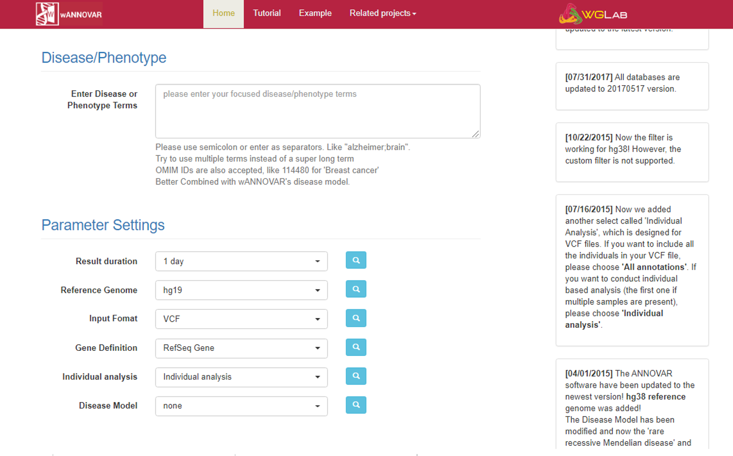
Finally, there are some Parameter Settings that can be modified:
- Result duration: it can now only be set to “1 day”, since your files will be automatically removed after 24 hours.
- Reference genome: you can choose between hg19 (GRCh37) and hg38 (GRCh38).
- Input Format: you can upload not only vcf files, but also other kinds of variant files.
- Gene Definition: the database you want to use for gene function annotation. Three oprtions are available: RefSeq, UCSC Known, ENSEMBL/Gencode
- Individual analysis: the “Individual analysis” option allows you to perform further filtering steps (based on the Disease/Phenotype terms or the Disease Model) on a single sample (if you upload a multisample vcf only the first sample will be considered); the “All Annotaions” option will annotate all variants in your multisample vcf, maintaining the original columns of your vcf as the last columns of your output file.
- Disease Model: this options allows for some basic filtering of your variants based on the expected mechanism of inheritance. In mainly consider frequencies, sample genotypes and consequences at level of genic function. FIltering step are summarized among the results and they are only performed on a single sample: the program does not perform any multisample evaluation (i.e.: variant segregation in a trio) and cannot classify any variant as de novo even if you provide a multisample vcf with parental genotypes.
Clinical databases for further manual variant annotation
Once you have obtained a file with the annotation of your variants, you might find useful to annotate also the involved genes, in order to know, for instance, the list of diseases that may be associated with them.
Some databases that can the jb are the following:
- The gene2phenotype dataset (G2P) integrates data on genes, variants and phenotypes for example relating to developmental disorders. In the “Download” section you will find both databases of genes related to cancer and to developmental disorders. Those files report for each gene listed: the OMIM number, the associated disease name, the disease OMIM number, the disease category (you can fing more details in the “Terminology” section), whether the disease is caused by biallelic or monoallelic variants (“allelic requirement”), the expected category of variant to be causative of the disease, and a few other details.
- In the “Download” section of the OMIM database, if you register for research and educational use, you may obtain different lists of OMIM genes and their associated phenotypes.
- Among the files available for download from the gnomAD database, you may get per-gene constraint scores (for further details, please check the paper by the Exome Aggregation Consortium on “Nature. 2016 Aug 18; 536(7616):285–291.”). Those score may indicate if a specific gene is expected to be intolerant to loss-of-function variants (pLI) (haploinsufficiency), or if it is predicted to be associate to recessive diseases.
In the end, you can add these annotations to your wANNOVAR files by using the VLOOKUP function in Excel.
CNV detection from targeted sequencing data
- Copy Number Variants (CNVs) are imbalances in the copy number of the genomic material that result in either DNA deletions (copy loss) or duplications
- CNVs can cause/predispose to human diseases by altering gene structure/dosage or by position effect
- CNV size ranges from 50 bp to megabases
- Classical methods to identify CNVs use array-based technologies (SNP/CGH)
- Computational approaches have been developed to identify CNVs in targeted sequencing data from hybrid capture experiments
Computational approaches
There are four main methods for CNV identification from short-read +NGS data (see figure below):
- Read Count (RC)
- Read Pair (RP)
- Split Read (SR)
-
De Novo Assembly (AS)
- RP and SR require continuous coverage of the CNV region or reads encompassing CNV breakpoints, as in whole genome sequencing. The sparse nature and small size of exonic targets hamper the application of these methods to targeted sequencing.
- RC is the best suited method for CNV detection from whole exomes or gene panels where:
- deletions appear as exonic targets devoid of reads
- duplications appear as exonic targets characterized by excess of coverage
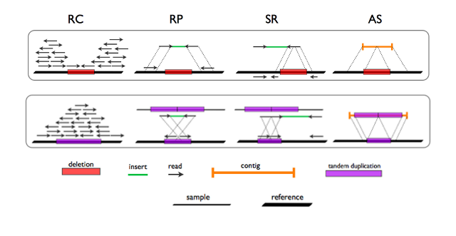
Figure 1. Methods for detection of CNVs in short read NGS data (adapted from Tattini et al., 2015)
RC method and data normalization
In targeted sequencing, a method to study DNA copy number variation by RC (as implemented in EXCAVATOR tool, Magi et al., 2013)) is to consider the exon mean read count (EMRC):
EMRC = RCe/Le
where RCe is the number of reads aligned to a target genomic region e and Le is the size of that same genomic region in base pairs (Magi et al., 2013)). Three major bias sources are known to affect EMRC dramatically in targeted sequencing data:
- local GC content percentage
- genomic mappability
- target region size
These biases contribute to non uniform read depth across target regions and, together with the sparse target nature, challenge the applicability of RC methods to targeted data. As shown in Figure 2 (left panel), in single-sample data the EMRC distributions of genomic regions characterized by different copy numbers largely overlap, revealing poor CNV prediction capability.
EMRC ratio between two samples can be used as a normalization procedure. The effect of EMRC ratio-based normalization is clear in Figure 2 (right panel) as a markedly improved correspondece between the predicted and the real copy number states.
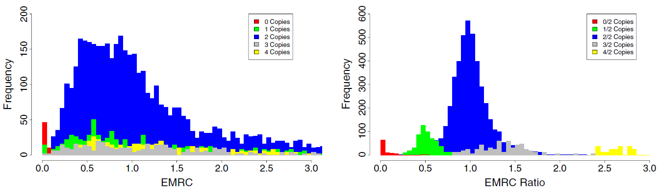
Figure 2. Effect of EMRC ratio on DNA copy number prediction (adapted from Magi et al., 2013)
Similarly FPKM, a normalized measure of read depth implemented in ExomeDepth tool (Plagnol et al., 2012), is affected by extensive exon–exon variability but comparison between pairs of exome datasets demonstrates high correlation level of the normalized read count data across samples making it possibile to use one or more combined exomes as reference set to base the CNV inference on (Plagnol et al., 2012).
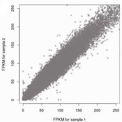
Figure 3. Correlation of the normalized read count data between samples (from Plagnol et al., 2012)
CNV detection accuracy
Strong correlation is observed between Affymetrix array-SNP and exome-derived data for CNVs >1 Mb (Figure 4, right panel), while including CNVs of any size dramatically decreases the correlation level (Figure 4, left panel). This can be explained by the different distribution of exons and SNP probes throughout the genome. Candidate CNV regions as identified by EXCAVATOR contain a comparable number of exons and SNP probes when they are > 1 Mb (R=0.8), while regions <100 Kb do not (R=-0.02). Accordingly, Krumm et al., 2012 report 94% precision in detecting CNVs across three or more exons.
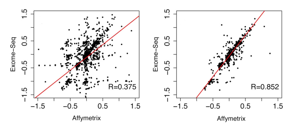
Figure 4. Correlation between array-SNP and exome-derived CNVs including all (left panel) or > 1 Mb CNVs (adapted from Magi et al., 2013)
To increase chances to detect CNVs encompassing few exons or in non-coding regions from exome data, D’Aurizio et al., 2016 have proposed an extension to EXCAVATOR to exploit off-target read count (EXCAVATOR2). Similar approaches taking advantage of off-target reads have been described by Bellos et al., 2014 or Talevich et al., 2016.
Tools for CNV detection from gene panels or exome data
A number of tools or pipelines implementing modified versions of previously published tools have been reported to detect single-exon CNVs in clinical gene panels:
In addition to the above-mentioned methods, many tools have been developed that detect CNVs from exomes. Evaluation of these tools is not straightforward as there is lack of a gold standard for comparison. As a consequence, there is no consensus level on pipelines as high as for single nucleotide variants. Zare et al., 2017 have reviewed this topic with focus on cancer, reporting poor overlap of different tools and added challenges for somatic variant calling.
hands_on Hands-on: CNV calling with ExomeDepth
ExomeDepth uses pairs of case and control exomes to identify copy number imbalances in case(s) compared to control(s). Here we provide a small data set including a pair of case/control BAM files and an exome target BED file restricted to a specific polymorphic region on chromosome 2q.
- CNV_case.bam.
- CNV_control.bam.
CNV_TruSeq_Chr2.bam
Your aim is to identify a large polymorphic deletion in case.
Regions of Homozygosity
- Runs of Homozygosity (ROHs) are sizeable stretches of consecutive homozygous markers encompassing genomic regions where the two haplotypes are identical
- Haplotypes in ROHs can underlie identity either by state (IBS) or by descent (IBD). IBD occurs when two haplotypes originate from a common ancestor (Figure 1), a condition whcih we refer to as autozygosity
- Autozygosity in an individual is the hallmark of high levels of genomic inbreeding (gF), often occurring in the offspring from consanguineous unions where parents are related as second-degree cousins or closer
- The most well-known medical impact of parental consanguinity is the increased risk of rare autosomal recessive diseases in the progeny, with excess risk inversely proportional to the disease-allele frequency (Bittles, 2001)
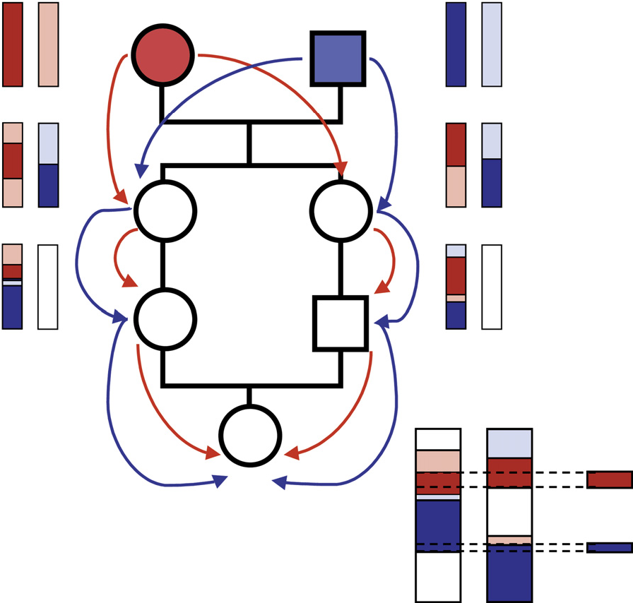 Figure 1. Schematic of haplotype flow along a consanguineous pedigrees to form autozygous ROHs in the progeny (from McQuillan et al., 2008)
Homozygosity mapping
- We refer to homozygosity mapping (Lander and Botstein, 1987) as an approach that infers autozygosity from the detection of long ROHs to map genes associated with recessive diseases
- A classical strategy to identify ROHs is based on SNP-array data and analysis with PLINK
- The combination of homozygosity mapping with exome sequencing has boosted genomic research and diagnosis of recessive diseases in recent years (Alazami et al., 2015; Monies et al., 2017)
- ROHs may be of clinical interest also since they can unmask uniparental isodisomy
- Computational approaches have been developed to identify ROHs directly in exome data, allowing simultaneous detection of variants and surrounding ROHs from the same datasets.
Computational approaches
As for CNVs, the sparse nature and small size of exonic targets are a challenge for the identification of continuous strethces of homozygous markers throughout the genome. This may affect the performance of tools originally tailored to SNPs when applied to exome data.
In Figure 2 a synthetic overview is given of algorithms, input data and output file types in bioinformatic tools for exome-based ROH detection. ROHs are divided in three size classes reflecting different mechanisms that have shaped them (according to Pemberton et al., 2012).
Usually, long ROH (approximately >1.5 Mb) arise as a result of close parental consanguinity, but also short-medium ROHs can be of medical interest in populations as involved in disease susceptibility, natural selection and founder effects (Ceballos et al., 2018).
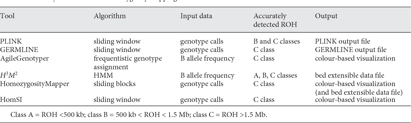 Figure 2. Summary of the tools for ROH detection from exome data (from Pippucci et al., 2014)
H3M2
H3M2 (Magi et al., 2014) is based on an heterogeneous Hidden Markov Model (HMM) that incorporates inter-marker distances to detect ROHs from exome data.
H3M2 calculates B-allele frequencies of a set of polymorphic sites throughout the exome as the ratio between allele B counts and the total read count at site i:
BAFi = Nb/N
H3M2 retrieves BAFi directly from BAM files to predict the heterozygous/homozygous genotype state at each polymorphic position i:
- when BAFi ~ 0 the predicted genotype is homozygous reference
- when BAFi ~ 0.5 the predicted genotype is heterozygous
- when BAFi ~ 1 the predicted genotype is homozygous alternative
H3M2 models BAF data by means of the HMM algorithm to discriminate between regions of homozygosity and non-homozygosity according to the BAF distribution along the genome (Figure 3).
 Figure 3. BAF data distribution Panels a, b and c show the distributions of BAF values against the genotype calls generated by the HapMap consortium on SNP-array data ( a ), the genotype calls made by SAMtools ( b ) and the genotype calls made by GATK ( c ). For each genotype caller, the distribution of BAF values is reported for homozygous reference calls (HMr), heterozygous calls (HT) and homozygous alternative calls (HMa). R is the Pearson correlation coefficient. Panels d–g show the distribution of BAF values in all the regions of the genome ( d ), in heterozygous regions ( e ), in homozygous regions ( f ) and in the X chromosome of male individuals ( g ). For each panel, the main plot reports the zoomed histogram, the left subplot shows the BAF values against genomic positions, whereas the right subplot shows the entire histogram of BAF values. (from Magi et al., 2014)
trophy Congratulations!
You successfully completed the advanced tutorial.
Contributors
- Tommaso Pippucci - Sant’Orsola-Malpighi University Hospital, Bologna, Italy
- Alessandro Bruselles - Istituto Superiore di Sanità, Rome, Italy
- Andrea Ciolfi - Ospedale Pediatrico Bambino Gesù, IRCCS, Rome, Italy
- Gianmauro Cuccuru - Albert Ludwigs University, Freiburg, Germany
- Giuseppe Marangi - Institute of Genomic Medicine, Fondazione Policlinico Universitario A. Gemelli IRCCS, Università Cattolica del Sacro Cuore, Roma, Italy
- Paolo Uva - IRCCS G. Gaslini, Genoa, Italy
Citing this Tutorial
- Alessandro Bruselles, Andrea Ciolfi, Gianmauro Cuccuru, Giuseppe Marangi, Paolo Uva, Tommaso Pippucci, 2020 Advanced data analysis of genomic data (Galaxy Training Materials). /clinical_genomics/advanced.html Online; accessed TODAY
- Batut et al., 2018 Community-Driven Data Analysis Training for Biology Cell Systems 10.1016/j.cels.2018.05.012
details BibTeX
@misc{-,
    author = "Alessandro Bruselles and Andrea Ciolfi and Gianmauro Cuccuru and Giuseppe Marangi and Paolo Uva and Tommaso Pippucci",
    title = "Advanced data analysis of genomic data (Galaxy Training Materials)",
    year = "2020",
    month = "10",
    day = "23"
    url = "\url{/clinical_genomics/advanced.html}",
    note = "[Online; accessed TODAY]"
}
@article{Batut_2018,
        doi = {10.1016/j.cels.2018.05.012},
        url = {https://doi.org/10.1016%2Fj.cels.2018.05.012},
        year = 2018,
        month = {jun},
        publisher = {Elsevier {BV}},
        volume = {6},
        number = {6},
        pages = {752--758.e1},
        author = {B{\'{e}}r{\'{e}}nice Batut and Saskia Hiltemann and Andrea Bagnacani and Dannon Baker and Vivek Bhardwaj and Clemens Blank and Anthony Bretaudeau and Loraine Brillet-Gu{\'{e}}guen and Martin {\v{C}}ech and John Chilton and Dave Clements and Olivia Doppelt-Azeroual and Anika Erxleben and Mallory Ann Freeberg and Simon Gladman and Youri Hoogstrate and Hans-Rudolf Hotz and Torsten Houwaart and Pratik Jagtap and Delphine Larivi{\`{e}}re and Gildas Le Corguill{\'{e}} and Thomas Manke and Fabien Mareuil and Fidel Ram{\'{\i}}rez and Devon Ryan and Florian Christoph Sigloch and Nicola Soranzo and Joachim Wolff and Pavankumar Videm and Markus Wolfien and Aisanjiang Wubuli and Dilmurat Yusuf and James Taylor and Rolf Backofen and Anton Nekrutenko and Björn Grüning},
        title = {Community-Driven Data Analysis Training for Biology},
        journal = {Cell Systems}
}
feedback Give us feedback on this content!
To give us feedback about these materials, or to get in touch with us, post a message in the forum https://groups.google.com/d/forum/sigu-training.